Chapter 10 Mersey IV - Catchments
10.1 Task 4: Extracting catchment characteristics
We know from the lecture that river hydrochemistry can be influenced by a range of catchment characteristics, including land cover, soil type, bedrock geology, topography, and rainfall. Before we undertake statistical analysis, our next step is to extract these characteristics for each of the 70 catchments in the mersey_watersheds file (.shp), so we can relate these to the Environment Agency water quality data collected at each of the 70 monitoring sites.
Information on these characteristics for the Mersey region can be obtained from the relevant files in the data pack, including:
mersey_LC[categorical], based on LCM2000 data;mersey_HOST[categorical] i.e., Hydrology of Soil Types;mersey_bedrock[categorical], sourced from the British Geological Survey;mersey_dem_fill[continuous], a digital elevation model (50 m spatial resolution);mersey_rainfall[continuous], annual average rainfall (mm a-1).
To simplify our analysis, I am going to walk you through the approach to calculate some of these variables, including the average of the continuous datasets (elevation, slope, aspect, rainfall).
For the categorical datasets (e.g., percentage of the each of the land cover / soil / bedrock classes present), I have provided you with the summary values, stored in data/practical_2/mersey_EA_characteristics.csv.
While extracting these values is an important part of the data cleaning-preparation process, it is time-consuming, requiring reclassification of each categorical raster (e.g., simplifying the number of classes and removing classes that are not present in the study area) and normalisation of the values based on catchment area. Given the focus of EMMC, this part has been removed to give you more time to focus on the statistical analysis and interpretation (as requested by previous student feedback), and to relate your results to key environmental concepts.
If you are interested in the reclassification approach, I have provided some guidance in the final chapter here.
10.1.1 Calculating surface derivatives
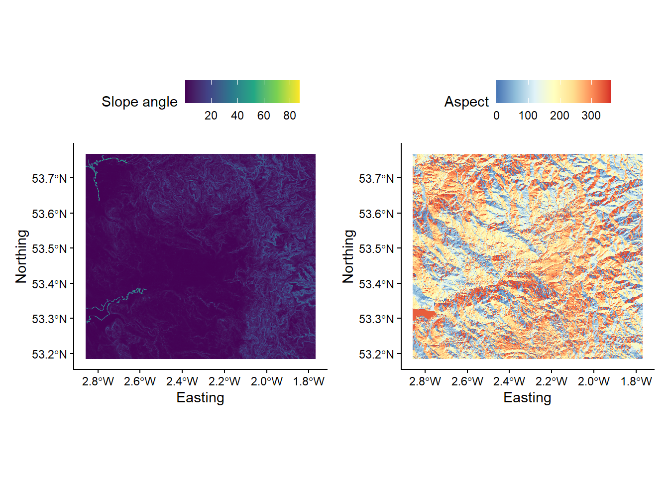
Before we can extract characteristics for each watershed, we need to produce some additional layers. Here, we are interested in the effects of elevation (the data from mersey_DEM_fill) and rainfall (mersey_rainfall), as well as topographic slope and aspect, both of which likely influence the path of water through the landscape. These two attributes (slope, aspect) are known as surface derivatives as they are calculated (derived) from the DEM.
To produce slope and aspect rasters:
use the
wbt_slopeandwbt_aspectfunctions, using the original filled DEM as the input data (mersey_dem_fill.tif) and using appropriate output names (e.g.mersey_dem_slopeandmersey_dem_aspect).
Your outputs should resemble the following:

10.1.2 Extracting continuous characteristics
To begin:
Load the
mersey_watersheds.shpfile into R (produced in Task 3) using thest_readfunction, storing in a variable calledwatersheds.
Next, print out attribute names for the shapefile as follows:
## [1] "FID" "VALUE" "geometry"For our analysis, the attribute of interest is VALUE, which contains the unique Environment Agency ID for each watershed. Importantly, this is also found in mersey_EA_chemisty.csv file. This will enable us to join the two datasets, populating the attribute table of the watersheds variable with the water quality measurements stored in the csv.
To simplify this, use the following code to replace the column name
VALUEwith a new nameSeed_Point_ID. The latter is used in themersey_EA_chemisty.csv.
# Replaces column name 'VALUE' with 'SEED_Point_ID'
names(watersheds)[names(watersheds) == 'VALUE'] <- 'Seed_Point_ID'
You can re-use the
colnamesfunction to check it worked correctly:
With this updated:
We can now load the Environment Agency data using
read.csv(), as shown in Chapter 3:
# Loads csv using read.csv
ea_data <- read.csv(here("data", "practical_2", "mersey_EA_chemistry.csv"))
and merge using the
mergefunction:
# Merge based upon matching Seed_Point_IDs
watersheds_ea <- merge(watersheds, ea_data, by = "Seed_Point_ID")
Use the
head()function to inspect the first few rows of our new data frame.
## Simple feature collection with 6 features and 14 fields
## Geometry type: MULTIPOLYGON
## Dimension:     XY
## Bounding box:  xmin: 343660.8 ymin: 382963.7 xmax: 353552.6 ymax: 394555.6
## Projected CRS: OSGB36 / British National Grid
##   Seed_Point_ID FID   EA_ID    Group   Ph   SSC     Ca    Mg  NH4  NO3  NO2  TON
## 1             1  54 1940214 Training 7.79 21.37  60.82 11.12 0.24 2.64 0.08 2.73
## 2             2  42 1941025  Testing 7.79 33.52  75.45 17.52 4.46 3.24 0.11 3.35
## 3             3  40 1941017 Training 8.55 11.69  58.54 20.50 0.25 0.83 0.02 0.84
## 4             4  47 1941007 Training 7.71 34.06  96.83 46.33 0.24 3.65 0.07 3.73
## 5             5  45 1941002 Training 8.08 70.81 141.98 85.85 0.40 4.47 0.05 4.52
## 6             6  44 1941003 Training 8.12 34.00 174.49 86.27 0.21 2.69 0.06 2.75
##    PO4    Zn                       geometry
## 1 0.34 50.00 MULTIPOLYGON (((345159.5 38...
## 2 0.99 20.51 MULTIPOLYGON (((348107.1 39...
## 3 0.07 35.23 MULTIPOLYGON (((346108.7 39...
## 4 0.21 74.26 MULTIPOLYGON (((350505.1 39...
## 5 0.14 20.16 MULTIPOLYGON (((351854 3906...
## 6 0.15 18.27 MULTIPOLYGON (((352903.1 39...
Save your script before continuing.
Before we move on to extract our continuous derivatives (average elevation, rainfall, slope and aspect), it is worth noting that R variables can be removed from the environment as follows:
This can be useful if R is running slowly.
To extract continuous derivatives, we are going to use the extract function from the raster package, which is described here. We’ll be using this function for each continuous dataset. It is also used for extracting categorical derivatives, as demonstrated here, so it’s important that you understand what it’s doing.
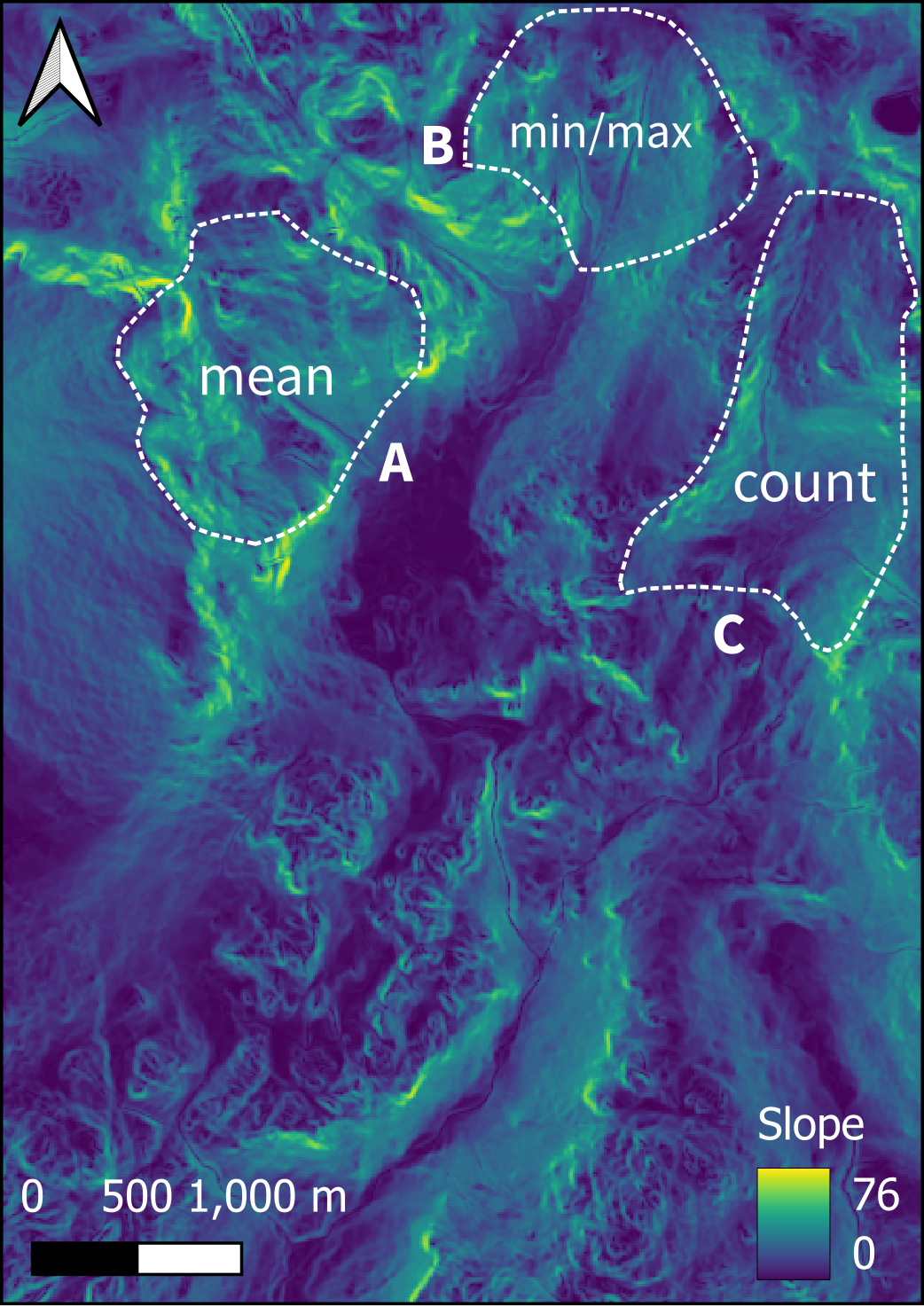
Broadly, the function extracts values from a raster object at the locations of spatial vector data, where the value of interest is user-defined. For example, this could be the mean (e.g. the average elevation of a DEM within a vector polygon), the count (e.g. the number of cells within a vector polygon), or a minimum or maximum (e.g. the maximum elevation within a vector polygon), as shown in the figure below:
Figure 5: Visual example of the extract function. In this example, our raster layer is the slope of the terrain in the Eskdale catchment, studied in Week 9, with values ranging from 0° (flat) to 76° (very steep). Our vector layer is a series of three \(Polygons\), covering three upland locations (other valid vector types include \(Points\) and \(Lines\)). Here, the extract function would return the average and minimum-maximum slope for \(Polygons\) \(A\) and \(B\) respectively, and the count (number of raster cells) for \(Polygon\) \(C\).
To use the extract function, the raster dataset needs to be loaded into R.
Load the digital elevation model into R and store with a sensible variable name e.g.
mersey_dem:
Now we can use the
extractfunction as follows. This takes in both raster (mersey_dem) and vector input data (watersheds_ea), where the value of interest is determined by thefunparameter (i.e. a function). Here we are using an existing base R function (e.g. mean) but we can use user-defined functions as well. For example,fun=function(x, ...) length(x)would count the length (or number) of raster cells for each watershed, andminormaxwould return the minimum and maximum elevations, respectively. In our case, we just want to calculate the mean (average) elevation, so we can use the approach below:
# Extracts raster values for each watershed, calculates mean (fun=mean), stores in attribute table ($average_elevation), with NA values removed (na.rm=TRUE)
watersheds_ea$average_elevation <- extract(mersey_dem, watersheds_ea, fun=mean, na.rm=TRUE)
When you’re happy you understand the process, load the other continuous rasters into R with sensible variable names (e.g.
mersey_rainfall,mersey_slope,mersey_aspect) and use theextractfunction to calculate the relevant attributes e.g.$average_rainfall,$average_slope,$average_aspect.
Use the
head()function to inspect the output.
10.1.3 Extracting categorical characteristics
As noted above, I have produced some catchments characteristics for you, derived from mersey_LC, mersey_HOST and mersey_bedrock. If you want to learn about the approach, it is detailed here. This information is stored in mersey_EA_characteristics.csv and includes:
- Percentage of the each of the five land cover classes present:
- Arable %
- Heath %
- Grassland %
- Urban %
- Wetland %
- Percentage of the each of the four soil types present:
- Permeable %
- Impermeable %
- Gleyed %
- Peats %
- Percentage of the each of the three bedrock geology types present:
- Sands_and_Muds %
- Limestone %
- Coal %
Load the above dataset using
read.csv()and then merge this dataset withwatersheds_ea(containing the continuous characteristics calculated above) using themergefunction andSeed_Point_IDas the merge value.
Again, use the
head()function to check this worked as expected.
To finish Task 4:
Run the following code, which removes the geometry stored in the data frame (not required for subsequent analysis) and saves our dataframe as a comma-separated file.
# Drops geometry attribute from watersheds_ea
watersheds_ea <- st_drop_geometry(watersheds_ea)

# Writes data frame to comma-separated file
write.csv(x = watersheds_ea, here("output", "practical_2", "mersey_watersheds_ea.csv"), row.names=FALSE)
To check your calculations:
Run
head(watersheds_ea), which should resemble the following:
##   Seed_Point_ID FID   EA_ID    Group   Ph   SSC     Ca    Mg  NH4  NO3  NO2  TON
## 1             1  54 1940214 Training 7.79 21.37  60.82 11.12 0.24 2.64 0.08 2.73
## 2             2  42 1941025  Testing 7.79 33.52  75.45 17.52 4.46 3.24 0.11 3.35
## 3             3  40 1941017 Training 8.55 11.69  58.54 20.50 0.25 0.83 0.02 0.84
## 4             4  47 1941007 Training 7.71 34.06  96.83 46.33 0.24 3.65 0.07 3.73
## 5             5  45 1941002 Training 8.08 70.81 141.98 85.85 0.40 4.47 0.05 4.52
## 6             6  44 1941003 Training 8.12 34.00 174.49 86.27 0.21 2.69 0.06 2.75
##    PO4    Zn average_elevation average_rainfall average_slope average_aspect
## 1 0.34 50.00          21.51344         539.8778     0.4947966       94.18135
## 2 0.99 20.51          39.95542         581.1832     1.2605843      205.45723
## 3 0.07 35.23          66.75006         591.3545     1.9887265      195.48206
## 4 0.21 74.26          44.82042         549.0123     0.5363760      140.63359
## 5 0.14 20.16          43.72755         557.1751     1.6656744      120.61153
## 6 0.15 18.27          49.89805         562.9039     1.1076461      118.44821
##   Arable_percent Heath_percent Grassland_percent Urban_percent Wetland_percent
## 1      23.881537             0          21.42407      49.46440               0
## 2      44.563367             0          23.93578      20.94381               0
## 3       2.862986             0          33.46967      35.71915               0
## 4      36.419753             0          10.08230      51.23457               0
## 5      62.289562             0          18.51852      19.19192               0
## 6      27.402135             0          10.85409      43.77224               0
##   Permeable_percent Impermeable_percent Gleyed_percent Peats_percent
## 1           0.00000                   0       64.90233     35.097669
## 2           6.59207                   0       84.23741      9.170518
## 3          19.90457                   0       80.09543      0.000000
## 4           0.00000                   0      100.00000      0.000000
## 5           0.00000                   0      100.00000      0.000000
## 6           0.00000                   0      100.00000      0.000000
##   Sands_and_Muds_percent Limestone_percent Coal_percent
## 1               89.09893                 0            0
## 2              100.00000                 0            0
## 3              100.00000                 0            0
## 4              100.00000                 0            0
## 5              100.00000                 0            0
## 6              100.00000                 0            0
If you wish, it might be good idea to clean / simplify our R environment before commencing the statistical analysis. To do so, best practice is to restart R (
Ctrl + Shift + F10on Windows) or you can use the following coderm(list = ls())to remove all objects from the workspace. While the latter isn’t a perfect solution (see here), it can be of value if used prudently.
