Chapter 8 Mersey II - Set-up
8.1 Practical overview
This practical is comprised of eight primary tasks, with three weeks of class time available (Weeks 10 - 12). Each of the steps is described in more detail in the remainder of this document. An outline of the key tasks is as follows:
Mersey III (Chapter 9): To complete in class in Week 10, and finish before the class in Week 11:
- Task 1: Flow routing
- Task 2: Seed points
- Task 3: Watershed delineation
Mersey IV (Chapter 10): To complete in class in Week 11, and finish before the class in Week 12:
- Task 4: Reclassification of categorical datasets
- Task 5: Calculating surface derivatives
- Task 6: Extracting surface derivatives
Mersey V (Chapter 11): To complete in class in Week 12:
- Task 7: Model building i.e. relating river water quality to catchment metrics
- Task 8: Model evaluation
Any class time remaining can be used to commence your practical report and ask any questions you may have before submission.
8.2 Install programs
You should have already installed R and RStudio. If not, please refer to the instructions here before continuing.
8.3 Download data
The data for this practical have already been downloaded here and can be found in data/practical_2. The directory structure is outlined in Chapter 2.
8.4 Data description
In Practical 1, we used a single raster file (dem_10m.tif) and visualised and assessed the outputs of a number of WBT functions (e.g. fill, breach, slope, pointer, flow accumulation).
In Practical 2, we are going to use a much wider range of input data, all of which use the British National Grid (BNG), a projected coordinate Reference System [EPSG:27700]. Alongside a few supplementary files (which you may wish to use for plotting), the key data are described here:
- Raster data (
.tif):mersey_dem_fill- a filled digital elevation model of the Mersey Basin;
mersey_rainfall- a raster of precipitation values;
mersey_bedrock- a categorical raster of bedrock geology types;
mersey_HOST- a categorical raster of soil types (Hydrology of Soil Types);
mersey_LC- a categorical raster of land cover classes, based on LCM2000 data;
- Vector data (
.shp):mersey_EA_sites- a point vector representing the locations of water quality monitoring stations. The attribute table contains a unique Environment Agency ID for each (
EA_ID):
- a point vector representing the locations of water quality monitoring stations. The attribute table contains a unique Environment Agency ID for each (
- Tables (
.csv):mersey_EA_chemisty- a comma-delimited table containing measurements for the following water quality indicators, as well as corresponding Environment Agency IDs:
- pH: acidity/alkalinity;
- SSC: suspended solids concentration (mg l−1);
- Ca: calcium (mg l−1);
- Mg: magnesium (mg l−1);
- NH4: ammonium (mg-N l−1);
- NO3: nitrate (mg-N l−1);
- NO2: nitrite (mg-N l−1);
- TON: total oxidised nitrogen (mg-N l−1);
- PO4: phosphate (mg-P l−1);
- Zn: zinc (μg l−1).
- a comma-delimited table containing measurements for the following water quality indicators, as well as corresponding Environment Agency IDs:
Read through the above descriptions carefully, making sure you understand the data we are using before moving on. We’ll be combining the Environment Agency measurements of water quality (e.g. pH, SSC, …) with spatial data representing the catchment (e.g. topography, rainfall, land cover, …) to investigate the controls on water quality across the Mersey Basin.
8.6 Projects and Scripts
8.6.1 Using an existing R project
In Practical 2 (Eskdale), we utilised an R Project called GEOG70581. Your GEOG70581 directory should resemble the following:
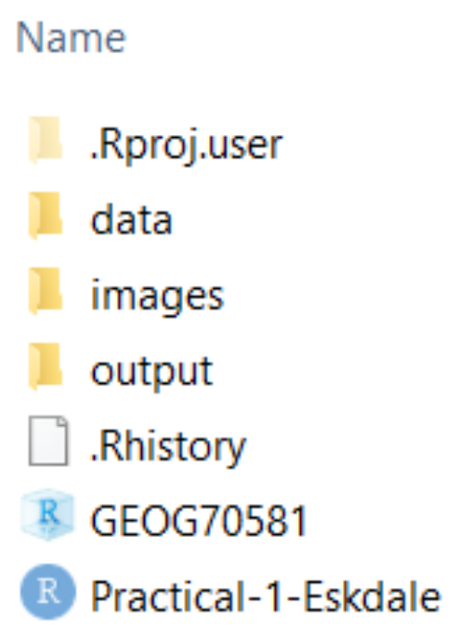
Here we have sub-directories for the original data (data) and any spatial data files or images we might create (output and images). We can also see the GEOG70581 project file and the Practical-1-Eskdale R script. The former is used to improve file access and to ensure our code is reproducible, self-contained and portable (see here for a refresher). The latter contains all our code and comments relating to Practical 1.
In this practical, we don’t need to create a new R project. We will simply use the existing R project as follows:
Go to File, Open Project in New Session, and select the GEOG70581 project file.
If this has been successful, your console should have been updated to include the path to your project working directory as follows:

8.6.2 Creating an R script
As shown in the file directory image above, we already have an R script for the Eskdale practical (Practical-1-Eskdale). As we are now working on a separate practical, with different input data and analytical techniques, it makes sense to create a new script to store the code and comments.
To create a new script for Practical 2:
Navigate to File, New File and R Script.
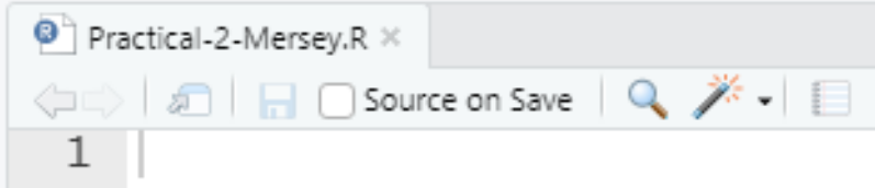
To save the script:
Navigate to File and Save As, and save it in the GEOG70581 folder with an appropriate name (e.g.
Practical-2-Mersey)
This should now resemble the following:
8.7 Loading packages
As we’re working in the same R project from Practical 1, we don’t need to re-install already utilised packages (e.g. whitebox).
However, we will need to install some new packages and ensure that all packages are loaded into the R environment.
Copy and paste the
check.packagesfunction into your new script, either from below or fromPractical-1-Eskdale.R:
# Function to check and install packages
check.packages <- function(pkg){
  new.pkg <- pkg[!(pkg %in% installed.packages()[, "Package"])]
  if (length(new.pkg))
    install.packages(new.pkg, dependencies = TRUE)
  sapply(pkg, require, character.only = TRUE)
}
In Practical 1, we used the following packages:
ggplot2- for data visualisation;
here- to construct paths to your project files;
raster- for reading, analysing and writing of raster and vector data;
sf- for simple storage of vector data;
ggspatial- for simple plotting of raster data in ggplot2;
whitebox- for geospatial analysis (a front-end for WhiteboxTools);
In Practical 2, we are going to use a number of additional packages:
data.table- for easy manipulation of tables;
dplyr- for easy manipulation of data frames;
forcats- for working with categorical variables (factors);
MASS- for statistical analysis, based upon Venables and Ripley (2002) “Modern Applied Statistics with S”;
units- for calculation of measurement units;
corrplotandolsrr- for correlation and regression analysis.
To load new packages, you can either use the install.packages() and library() functions or more simply, add package names to the packages vector, as shown here:
# Checks and installs packages
packages <- c("ggplot2", "ggspatial", "here", "raster", "sf", "whitebox", # Practical-1
              "data.table", "dplyr", "forcats", "MASS", "units") # Practical-2
check.packages(packages)
Use the above code to install and load the required packages.